Music Authorship
Find this notebook at
EpyNN/epynnlive/author_music/prepare_dataset.ipynb.Regular python code at
EpyNN/epynnlive/author_music/prepare_dataset.py.
Run the notebook online with Google Colab.
Level: Advanced
This notebook is part of the series on preparing data for Neural Network regression with EpyNN.
It deals with a real world problem and therefore will focus on the problem itself, rather than basics that were reviewed along with the preparation of the following dummy dataset:
Authorship prediction of artistic content
Detection of fake art is a challenge for a market reportedly costing more than 60 billion USD per year. Indeed, the price of an art piece is directly linked to its author and the more famous one author is, the more falsifications are to be expected. You might like to visit Deep learning approaches to pattern extraction and recognition in paintings and drawings for an overview of deep learning methods used to assign one painting to the corresponding author.
Herein, we are going to work with audio art or music. More specifically, we will prepare one True and False dataset from audio .wav files that may have been produced by one author or another. The goal will be to train a model able to predict, for one piece of music, which of the True or False authors is playing.
Note that by one author or another, in the context of this notebook, we do not necessarily mean that “author-specific” patterns in data are directly related to one author’s style. Herein we make things simple, although “author-specific” patterns may include style, background noise, specific guitar model, etc…
Prepare music clips from .wav files
Audio files can contain music of any duration. Moreover, we may just have a single audio file for each of the True and False authors. Among other reasons, we therefore need to make clips to have more than one training example per author.
Imports
[1]:
# EpyNN/epynnlive/author_music/prepare_dataset.ipynb
# Install dependencies
!pip3 install --upgrade-strategy only-if-needed epynn

# Standard library imports
import tarfile
import random
import glob
import os

# Related third party imports
import wget
import numpy as np
import matplotlib.pyplot as plt
from scipy.io import wavfile

# Local application/library specific imports
from epynn.commons.logs import process_logs
Note the tarfile which is a Python built-in standard library and the first choice to deal with .tar archives and related.
Note the import of wavfile from scipy.io. Scipy is a “Python-based ecosystem of open-source software for mathematics, science, and engineering” while the wavfile module provides easy-to-use read/write functions for audio .wav files.
[2]:
### Seeding
[3]:
random.seed(1)
For reproducibility.
Clip music
By clipping music we mean make chunks of it. We need a TIME for one clip, which defaults to 1 second.
Also, we will resample the data, because the .wav file has sampling rate of 44100 Hz which means 44100 data points per second. This is a lot when considering that we will later retrieve many clips of one second. Indeed, while one .wav file weights only a few MB, it weights much more when embedded into NumPy arrays. To prevent overloading the RAM, we need to reduce the number of data points per clip. This SAMPLING_RATE defaults to 10000 Hz and as a consequence we will lose most of the
patterns with frequencies is higher than 5000 Hz (See Nyquist rate for more).
Fortunately, the highest pitch a guitar can play is lower than 5000 Hz (See Range (music) for more). Although harmonics can go beyond this limit, we can expect to not lose the patterns or signatures for each of the True and False authors.
For the sake of rigor, note that when saying resampling - downsampling - we mean decimation instead. See Downsampling (signal processing) for more details. In brief, a complete scheme for downsampling requires applying a lowpass filter to eliminate high frequencies and then proceeding with the decimation process. In the context of this example the impact of not applying a low pass filter is limited, and so we choose to only apply decimation for the sake of simplicity.
[7]:
def clips_music(wav_file, TIME=1, SAMPLING_RATE=10000):
    """Clip music and proceed with resampling.

    :param wav_file: The filename of .wav file which contains the music.
    :type wav_file: str

    :param SAMPLING_RATE: Sampling rate (Hz), default to 10000.
    :type SAMPLING_RATE: int

    :param TIME: Sampling time (s), defaults to 1.
    :type TIME: int

    :return: Clipped and re-sampled music.
    :rtype: list[:class:`numpy.ndarray`]
    """
    # Number of features describing a sample
    N_FEATURES = int(SAMPLING_RATE * TIME)

    # Retrieve original sampling rate (Hz) and data
    wav_sampling_rate, wav_data = wavfile.read(wav_file)

    # 16-bits wav files - Pass all positive and norm. [0, 1]
    # wav_data = (wav_data + 32768.0) / (32768.0 * 2)
    wav_data = wav_data.astype('int64')
    wav_data = (wav_data + np.abs(np.min(wav_data)))
    wav_data = wav_data / np.max(wav_data)

    # Digitize in 4-bits signal
    n_bins = 16
    bins = [i / (n_bins - 1) for i in range(n_bins)]
    wav_data = np.digitize(wav_data, bins, right=True)

    # Compute step for re-sampling
    sampling_step = int(wav_sampling_rate / SAMPLING_RATE)

    # Re-sampling to avoid memory allocation errors
    wav_resampled = wav_data[::sampling_step]

    # Total duration (s) of original data
    wav_time = wav_data.shape[0] / wav_sampling_rate

    # Number of clips to slice from original data
    N_CLIPS = int(wav_time / TIME)

    # Make clips from data
    clips = [wav_resampled[i * N_FEATURES:(i+1) * N_FEATURES] for i in range(N_CLIPS)]

    return clips
In addition to clipping and resampling, we have done the following signal normalization within [0, 1]: Audio files 16-bits encoded are lists of integers ranging from -32768 , +32767 for a total of 2^16 bins. We need to normalize within [0, 1] for one technical reason: such high values are likely to generate floating point errors when passed through exponential functions, among others.
[8]:
print(np.exp(32767))
inf
/usr/local/lib/python3.7/dist-packages/ipykernel_launcher.py:1: RuntimeWarning: overflow encountered in exp
  """Entry point for launching an IPython kernel.
Normalization was achieved on a per-file basis, because we assume that sound level extrema may be different from one recording to the other or from one author to the other. Therefore, the minimum and maximum sound level from one file to the NumPy array will be equal to zero and one, respectively, after normalization. In addition to preventing floating point errors, this helps to make further network training faster because the network does not need to perform such normalization by itself.
The last thing we have done is signal re-digitalization using a 4-bits encoder over 16 bins. This is because we make the choice to later one-hot encode these data. When doing the latter, we lose information over signal amplitude and we focus on patterns in signal.
Note that:
One-hot encoding does reasonably apply on digitized data only. More general, it does apply on data encoded over a given, limited number of semantic units (including bins, characters, words and so on).
In the context of this notebook, signal normalization is not necessary if applying one-hot encoding. It may still be done, but mostly for convenience.
See One-hot encoding of string features for details about the process. Note that while one-hot encoding is mandatory when dealing with string input data, it can also be done with digitized numerical data as is the case here.
We can now see how it looks with different settings for the same clip length of 0.1s:
[9]:
fig, ax = plt.subplots(2, 2, sharey=True)

clips = clips_music(wav_test, TIME=0.1, SAMPLING_RATE=44100)
ax[0, 0].plot(clips[5])
ax[0, 0].set_title('44100 Hz')

clips = clips_music(wav_test, TIME=0.1, SAMPLING_RATE=11025)
ax[0, 1].plot(clips[5])
ax[0, 1].set_title('11025 Hz')

clips = clips_music(wav_test, TIME=0.1, SAMPLING_RATE=900)
ax[1, 0].plot(clips[5])
ax[1, 0].set_title('900 Hz')

clips = clips_music(wav_test, TIME=0.1, SAMPLING_RATE=100)
ax[1, 1].plot(clips[5])
ax[1, 1].set_title('100 Hz')

plt.tight_layout()
plt.show()
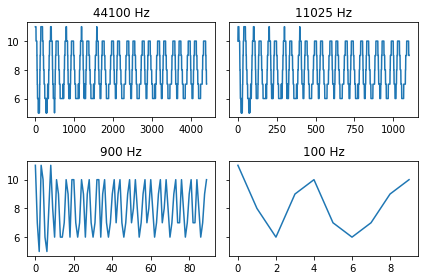
Along with decreasing the sampling rate, we observe that patterns corresponding to higher frequencies are eliminated.
Prepare dataset
Below is a function we use to prepare the labeled dataset.
[10]:
def prepare_dataset(N_SAMPLES=100):
    """Prepare a dataset of clipped music as NumPy arrays.

    :param N_SAMPLES: Number of clip samples to retrieve, defaults to 100.
    :type N_SAMPLES: int

    :return: Set of sample features.
    :rtype: tuple[:class:`numpy.ndarray`]

    :return: Set of single-digit sample label.
    :rtype: tuple[:class:`numpy.ndarray`]
    """
    # Initialize X and Y datasets
    X_features = []
    Y_label = []

    wav_paths = os.path.join('data', '*', '*wav')

    wav_files = glob.glob(wav_paths)

    # Iterate over WAV_FILES
    for wav_file in wav_files:

        # Retrieve clips
        clips = clips_music(wav_file)

        # Iterate over clips
        for features in clips:

            # Clip is positive if played by true author (0) else negative (1)
            label = 0 if 'true' in wav_file else 1

            # Append sample features to X_features
            X_features.append(features)

            # Append sample label to Y_label
            Y_label.append(label)

    # Prepare X-Y pairwise dataset
    dataset = list(zip(X_features, Y_label))

    # Shuffle dataset
    random.shuffle(dataset)

    # Truncate dataset to N_SAMPLES
    dataset = dataset[:N_SAMPLES]

    # Separate X-Y pairs
    X_features, Y_label = zip(*dataset)

    return X_features, Y_label
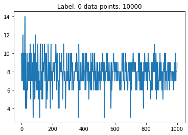
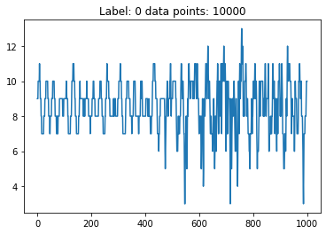
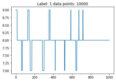
Let’s check the function.
[11]:
X_features, Y_label = prepare_dataset(N_SAMPLES=5)

for features, label in zip(X_features, Y_label):
    plt.plot(features[:features.shape[0] // 10])
    plt.title('Label: %s data points: %s' % (label, features.shape[0]))
    plt.show()
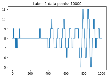
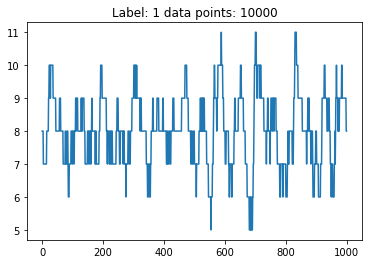
We are ready to proceed with the training of a network based on these data.
Live examples
The function prepare_dataset() presented herein is used in the following live examples:
Notebook at
EpyNN/epynnlive/author_music/train.ipynbor following this link.Regular python code at
EpyNN/epynnlive/author_music/train.py.