Basics with string sequence
Find this notebook at
EpyNN/epynnlive/dummy_string/train.ipynb.Regular python code at
EpyNN/epynnlive/dummy_string/train.py.
Run the notebook online with Google Colab.
Level: Beginner
In this notebook we will review:
Handling sequential string data.
Training of Feed-Forward (FF) and recurrent networks (RNN, LSTM, GRU).
Differences between decisions and probabilities and related functions.
It is assumed that all basics notebooks were already reviewed:
This notebook does not enhance, extend or replace EpyNN’s documentation.
Relevant documentation pages for the current notebook:
Environment and data
Follow this link for details about data preparation.
Briefly, these dummy string data consist of sequences of characters. Sample features are each represented by one sequence and can be either associated with a positive or negative label.
Positive sequences are met when the first element in the sequence is equal to the last element in this same sequence, and reciprocally.
[1]:
# EpyNN/epynnlive/dummy_string/train.ipynb
# Install dependencies
!pip3 install --upgrade-strategy only-if-needed epynn

# Standard library imports
import random

# Related third party imports
import numpy as np

# Local application/library specific imports
import epynn.initialize
from epynn.commons.io import one_hot_decode_sequence
from epynn.commons.maths import relu, softmax
from epynn.commons.library import (
    configure_directory,
    read_model,
)
from epynn.network.models import EpyNN
from epynn.embedding.models import Embedding
from epynn.flatten.models import Flatten
from epynn.rnn.models import RNN
from epynn.gru.models import GRU
from epynn.lstm.models import LSTM
from epynn.dense.models import Dense
from epynnlive.dummy_string.prepare_dataset import prepare_dataset
from epynnlive.dummy_string.settings import se_hPars


########################## CONFIGURE ##########################
random.seed(1)

np.set_printoptions(threshold=10)

np.seterr(all='warn')

configure_directory()


############################ DATASET ##########################
X_features, Y_label = prepare_dataset(N_SAMPLES=480)
Let’s control what we retrieved.
[2]:
print(len(X_features))
print(len(X_features[0]))
print(X_features[0])
print(Y_label[0])
480
12
['G', 'A', 'C', 'T', 'T', 'G', 'G', 'C', 'C', 'A', 'T', 'C']
1
We retrieved a set of sample features describing 480 samples.
Each sample is described by 12 string features.
Herein the label is 1 because the first and last element are different.
Feed-Forward (FF)
To compare Feed-Forward and recurrent networks, we are going to train a simple Perceptron first.
Embedding
The principle of One-hot encoding of string features was detailed before.
Briefly, we can not do math on string data. Therefore, the one-hot encoding process may be summarized as such:
List of all elements of size vocab_size. This basically answers: what is the number of distinct elements we can find in your data?
Each element is associated with one index in the range(0, vocab_size). This provides an
element_to_idxencoder.For one sample and for each element in the associated list of features, a zero array is initialized. This array is set to one at the index which is assigned to the
element_to_idxencoder.
This is achieved during instantiation of the embedding layer by setting up X_encode=True.
[3]:
embedding = Embedding(X_data=X_features,
                      Y_data=Y_label,
                      X_encode=True,
                      Y_encode=True,
                      relative_size=(2, 1, 0))
Let’s inspect some properties.
[4]:
print(embedding.e2i)  # element_to_idx
print(embedding.dtrain.X[0])

print(embedding.i2e)  # idx_to_element
print(one_hot_decode_sequence(embedding.dtrain.X[0], embedding.i2e))
{'A': 0, 'C': 1, 'G': 2, 'T': 3}
[[0. 0. 1. 0.]
 [1. 0. 0. 0.]
 [0. 1. 0. 0.]
 ...
 [1. 0. 0. 0.]
 [0. 0. 0. 1.]
 [0. 1. 0. 0.]]
{0: 'A', 1: 'C', 2: 'G', 3: 'T'}
['G', 'A', 'C', 'T', 'T', 'G', 'G', 'C', 'C', 'A', 'T', 'C']
Encoded sequences may be decoded as shown above.
Flatten-Dense - Perceptron
Let’s inspect the shape of the data.
[5]:
print(embedding.dtrain.X.shape)
(320, 12, 4)
It contains 320 samples (m), each described by a sequence of 12 features (s) containing 4 elements (v).
12 features is the length of the sequences and 4 elements is the size of the vocabulary. Remember one-hot encoding makes a zero array of this size and sets 1 at the index corresponding to the element being encoded.
Still, the fully-connected or dense layer can only process bi-dimensional input arrays. That is the reason why we need to invoke a flatten layer in between the embedding and dense layer.
[6]:
name = 'Flatten_Dense-2-softmax'

se_hPars['learning_rate'] = 0.001

flatten = Flatten()

dense = Dense(2, softmax)

layers = [embedding, flatten, dense]

model = EpyNN(layers=layers, name=name)
Initialize using most classically a MSE or Binary Cross Entropy loss function.
[7]:
model.initialize(loss='BCE', seed=1, se_hPars=se_hPars.copy(), end='\r')
--- EpyNN Check OK! ---
Train for hundred epochs.
[8]:
model.train(epochs=50, init_logs=False)
Epoch 49 - Batch 0/0 - Accuracy: 0.738 Cost: 0.55582 - TIME: 2.14s RATE: 2.34e+01e/s TTC: 0s

+-------+----------+----------+-------+--------+-------+------------------------------------+
| epoch |  lrate   | accuracy |       |  BCE   |       |             Experiment             |
|       |  Dense   |  dtrain  | dval  | dtrain | dval  |                                    |
+-------+----------+----------+-------+--------+-------+------------------------------------+
|   0   | 1.00e-03 |  0.688   | 0.694 | 0.631  | 0.640 | 1635014418_Flatten_Dense-2-softmax |
|   5   | 1.00e-03 |  0.716   | 0.731 | 0.609  | 0.620 | 1635014418_Flatten_Dense-2-softmax |
|  10   | 1.00e-03 |  0.719   | 0.750 | 0.596  | 0.609 | 1635014418_Flatten_Dense-2-softmax |
|  15   | 1.00e-03 |  0.728   | 0.750 | 0.585  | 0.601 | 1635014418_Flatten_Dense-2-softmax |
|  20   | 1.00e-03 |  0.728   | 0.750 | 0.577  | 0.595 | 1635014418_Flatten_Dense-2-softmax |
|  25   | 1.00e-03 |  0.734   | 0.756 | 0.571  | 0.590 | 1635014418_Flatten_Dense-2-softmax |
|  30   | 1.00e-03 |  0.734   | 0.756 | 0.566  | 0.587 | 1635014418_Flatten_Dense-2-softmax |
|  35   | 1.00e-03 |  0.734   | 0.762 | 0.562  | 0.585 | 1635014418_Flatten_Dense-2-softmax |
|  40   | 1.00e-03 |  0.734   | 0.762 | 0.559  | 0.583 | 1635014418_Flatten_Dense-2-softmax |
|  45   | 1.00e-03 |  0.734   | 0.756 | 0.557  | 0.582 | 1635014418_Flatten_Dense-2-softmax |
|  49   | 1.00e-03 |  0.741   | 0.756 | 0.555  | 0.581 | 1635014418_Flatten_Dense-2-softmax |
+-------+----------+----------+-------+--------+-------+------------------------------------+
Plot the results.
[9]:
model.plot(path=False)
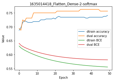
Strictly speaking, the Perceptron seems to have converged in the right direction.
By reducing the learning rate, all other things being equal, we obtained greater accuracy, lower cost and smoother curves on the plot.
You may have observed something possibly counter-intuitive:
The cost, which describes the mean difference between output probabilities and labels, is lower for the validation set compared to training set.
The accuracy, which describes the mean difference between output decisions and labels, is higher for the validation set compared to training set.
While the cost says the error is higher when evaluating on the validation set, the accuracy says the opposite.
That’s because accuracy compares decisions and labels, whereas the cost from the loss function compares probabilities and labels.
For code, maths and pictures behind the Flatten and Dense layers, follow these links:
Let’s take a break and understand the difference in addition to making clear some semantics.
Difference between accuracy and cost
The question is: Can we expect identical costs for the training and validation set if the accuracy is identical for the training and validation set?
Let’s compare what outputs from the dense layer (A) to the set of sample label (Y).
[10]:
# This is probability distributions for each sample.
print(model.embedding.dtrain.A)
print(model.embedding.dtrain.A.shape)

# These are the labels we target
print(model.embedding.dtrain.Y)
print(model.embedding.dtrain.Y.shape)
[[0.24990897 0.75009103]
 [0.15080179 0.84919821]
 [0.28627148 0.71372852]
 ...
 [0.09204908 0.90795092]
 [0.15813641 0.84186359]
 [0.41724774 0.58275226]]
(320, 2)
[[0. 1.]
 [0. 1.]
 [1. 0.]
 ...
 [1. 0.]
 [0. 1.]
 [0. 1.]]
(320, 2)
We have probabilities (A) versus binary values (Y).
To compute the accuracy, one needs to convert probabilities to decisions, as well as to retrieve single-digit labels.
[11]:
print(np.argmax(model.embedding.dtrain.A, axis=1))

# Equivalent to calling model.embedding.dtrain.y directly
print(np.argmax(model.embedding.dtrain.Y, axis=1))
[1 1 1 ... 1 1 1]
[1 1 0 ... 0 1 1]
Then, accuracy is computed such as:
[12]:
print ((np.argmax(model.embedding.dtrain.A, axis=1) == model.embedding.dtrain.y))
print ((np.argmax(model.embedding.dtrain.A, axis=1) == model.embedding.dtrain.y).mean())
[ True  True False ... False  True  True]
0.740625
The cost is computed from probabilities, not from decisions. This apart from the fact that accuracy and cost are simply two different functions.
To compute a cost, we first need to compute the loss, which provides information for each single probability in the array (A).
[13]:
# This is the cost. It deals with "true" labels against probabilities

loss = model.training_loss(model.embedding.dtrain.Y, model.embedding.dtrain.A)

print(loss.shape)
(320,)
The cost is a form of average of the loss. Whereas the loss is an array from element-wise comparison between probabilities and labels, the cost is a scalar which is an average per sample, itself an average of the element-wise loss for this sample.
[14]:
print(loss.shape)          # Averaged for each sample
print(loss.mean().shape)   # Average of above - scalar

cost = loss.mean()

print(cost)
(320,)
()
0.5554707080208504
Note that what is fed back in the network during the backward propagation phase is not the loss. It is the derivative of the loss.
[15]:
dloss = model.training_loss(model.embedding.dtrain.Y, model.embedding.dtrain.A, deriv=True)

print(loss)
print(dloss)    # dloss is referred to as dA
[0.2875607  0.16346266 1.2508147  ... 2.38543339 0.17213728 0.53999313]
[[ 0.66658576 -0.66658576]
 [ 0.58879069 -0.58879069]
 [-1.74659385  1.74659385]
 ...
 [-5.43188494  5.43188494]
 [ 0.59392045 -0.59392045]
 [ 0.85799753 -0.85799753]]
The loss function and derivatives natively provided with EpyNN can be found in EpyNN/epynn/commons/loss.py.
The metrics natively provided with EpyNN can be found in EpyNN/epynn/commons/metrics.py.
Recurrent Architectures
Herein, we are going to chain simple schemes based on recurrent architectures.
There are three most commonly cited recurrent layers:
Recurrent Neural Network (RNN): This is the most simple recurrent layer. It is composed of one to many recurrent units. Each cell performs a single activation which outputs the hidden cell state or simply hidden state.
Long Short-Term Memory (LSTM): By contrast with the RNN cell, the LSTM cell requires four activations which correspond to three different gates: forget, input (two activations), and output. To compute the hidden cell state, it then requires a fifth activation. Note that in addition to the hidden cell state, there is another so-called cell memory state.
Gated Recurrent Unit (GRU): Compared to the LSTM cell, the GRU cell has only two gates: reset and update. Practically talking, GRU trains faster than LSTM and is reported to perform better on small datasets or shorter sequences. Both GRU and LSTM, however, are state-of-the-art architectures to deal with sequential data.
See here for more detailed practical descriptions or simply via the pages linked on top of this notebook.
Embedding
In this example, we use the same setup as for Feed-Forward networks.
[16]:
embedding = Embedding(X_data=X_features,
                      Y_data=Y_label,
                      X_encode=True,
                      Y_encode=True,
                      relative_size=(2, 1, 0))
We can now chain the simplest schemes to train binary classifiers based on recurrent layers.
RNN-Dense
The number of RNN units in the RNN layer is set to 1.
[17]:
name = 'RNN-1_Dense-2-softmax'

se_hPars['learning_rate'] = 0.001

rnn = RNN(1)

dense = Dense(2, softmax)

layers = [embedding, rnn, dense]

model = EpyNN(layers=layers, name=name)
Initialize the model.
[18]:
model.initialize(loss='BCE', seed=1, se_hPars=se_hPars.copy(), end='\r')
--- EpyNN Check OK! ---
Train for 50 epochs.
[19]:
model.train(epochs=10, init_logs=False)
Epoch 9 - Batch 0/0 - Accuracy: 0.734 Cost: 0.58678 - TIME: 0.94s RATE: 1.06e+01e/s TTC: 0s

+-------+----------+----------+----------+-------+--------+-------+----------------------------------+
| epoch |  lrate   |  lrate   | accuracy |       |  BCE   |       |            Experiment            |
|       |   RNN    |  Dense   |  dtrain  | dval  | dtrain | dval  |                                  |
+-------+----------+----------+----------+-------+--------+-------+----------------------------------+
|   0   | 1.00e-03 | 1.00e-03 |  0.544   | 0.581 | 0.676  | 0.659 | 1635014422_RNN-1_Dense-2-softmax |
|   1   | 1.00e-03 | 1.00e-03 |  0.734   | 0.762 | 0.648  | 0.630 | 1635014422_RNN-1_Dense-2-softmax |
|   2   | 1.00e-03 | 1.00e-03 |  0.734   | 0.762 | 0.629  | 0.610 | 1635014422_RNN-1_Dense-2-softmax |
|   3   | 1.00e-03 | 1.00e-03 |  0.734   | 0.762 | 0.615  | 0.595 | 1635014422_RNN-1_Dense-2-softmax |
|   4   | 1.00e-03 | 1.00e-03 |  0.734   | 0.762 | 0.605  | 0.585 | 1635014422_RNN-1_Dense-2-softmax |
|   5   | 1.00e-03 | 1.00e-03 |  0.734   | 0.762 | 0.598  | 0.577 | 1635014422_RNN-1_Dense-2-softmax |
|   6   | 1.00e-03 | 1.00e-03 |  0.734   | 0.762 | 0.593  | 0.571 | 1635014422_RNN-1_Dense-2-softmax |
|   7   | 1.00e-03 | 1.00e-03 |  0.734   | 0.762 | 0.589  | 0.566 | 1635014422_RNN-1_Dense-2-softmax |
|   8   | 1.00e-03 | 1.00e-03 |  0.734   | 0.762 | 0.587  | 0.563 | 1635014422_RNN-1_Dense-2-softmax |
|   9   | 1.00e-03 | 1.00e-03 |  0.734   | 0.762 | 0.585  | 0.560 | 1635014422_RNN-1_Dense-2-softmax |
+-------+----------+----------+----------+-------+--------+-------+----------------------------------+
You may already note that results are virtually identical to just using a basic Perceptron, although slightly better.
[20]:
model.plot(path=False)
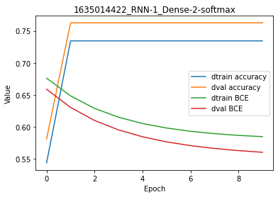
While the y-scale on the plot is a bit misleading when looking at the accuracy, there is no overfitting in there because the BCE cost is the same for both training and validation set at the end of the regression.
For code, maths and pictures behind the RNN layer, follow this link:
LSTM-Dense
Let’s now proceed with an LSTM layer composed of the 1 unit, all other things being equal.
[21]:
name = 'LSTM-1_Dense-2-softmax'

se_hPars['learning_rate'] = 0.005

lstm = LSTM(1)

dense = Dense(2, softmax)

layers = [embedding, lstm, dense]

model = EpyNN(layers=layers, name=name)
Initialize the model.
[22]:
model.initialize(loss='BCE', seed=1, se_hPars=se_hPars.copy(), end='\r')
--- EpyNN Check OK! ---
Train for 50 epochs.
[23]:
model.train(epochs=10, init_logs=False)
Epoch 9 - Batch 0/0 - Accuracy: 0.734 Cost: 0.57893 - TIME: 0.97s RATE: 1.03e+01e/s TTC: 0s

+-------+----------+----------+----------+-------+--------+-------+-----------------------------------+
| epoch |  lrate   |  lrate   | accuracy |       |  BCE   |       |            Experiment             |
|       |   LSTM   |  Dense   |  dtrain  | dval  | dtrain | dval  |                                   |
+-------+----------+----------+----------+-------+--------+-------+-----------------------------------+
|   0   | 5.00e-03 | 5.00e-03 |  0.734   | 0.762 | 0.586  | 0.563 | 1635014423_LSTM-1_Dense-2-softmax |
|   1   | 5.00e-03 | 5.00e-03 |  0.734   | 0.762 | 0.580  | 0.552 | 1635014423_LSTM-1_Dense-2-softmax |
|   2   | 5.00e-03 | 5.00e-03 |  0.734   | 0.762 | 0.579  | 0.550 | 1635014423_LSTM-1_Dense-2-softmax |
|   3   | 5.00e-03 | 5.00e-03 |  0.734   | 0.762 | 0.579  | 0.549 | 1635014423_LSTM-1_Dense-2-softmax |
|   4   | 5.00e-03 | 5.00e-03 |  0.734   | 0.762 | 0.579  | 0.549 | 1635014423_LSTM-1_Dense-2-softmax |
|   5   | 5.00e-03 | 5.00e-03 |  0.734   | 0.762 | 0.579  | 0.549 | 1635014423_LSTM-1_Dense-2-softmax |
|   6   | 5.00e-03 | 5.00e-03 |  0.734   | 0.762 | 0.579  | 0.549 | 1635014423_LSTM-1_Dense-2-softmax |
|   7   | 5.00e-03 | 5.00e-03 |  0.734   | 0.762 | 0.579  | 0.549 | 1635014423_LSTM-1_Dense-2-softmax |
|   8   | 5.00e-03 | 5.00e-03 |  0.734   | 0.762 | 0.579  | 0.549 | 1635014423_LSTM-1_Dense-2-softmax |
|   9   | 5.00e-03 | 5.00e-03 |  0.734   | 0.762 | 0.579  | 0.549 | 1635014423_LSTM-1_Dense-2-softmax |
+-------+----------+----------+----------+-------+--------+-------+-----------------------------------+
The accuracy metrics are simply identical to what we have seen with a simple RNN, which is much faster to compute. It is not significantly better than what we obtained from a simple Perceptron, itself way faster to compute than the RNN based network.
[24]:
model.plot(path=False)
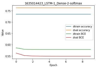
By contrast with the RNN-based network, we observe here a slight overfitting because the cost is lower for the training dataset compared to the validation dataset.
For code, maths and pictures behind the LSTM layer, follow this link:
GRU-Dense
Let’s now proceed with a GRU layer, all other things being equal.
[25]:
name = 'GRU-1_Dense-2-softmax'

se_hPars['learning_rate'] = 0.005

gru = GRU(1)

flatten = Flatten()

dense = Dense(2, softmax)

layers = [embedding, gru, dense]

model = EpyNN(layers=layers, name=name)
Initialize the network.
[26]:
model.initialize(loss='BCE', seed=1, se_hPars=se_hPars.copy(), end='\r')
--- EpyNN Check OK! ---
Train for 50 epochs.
[27]:
model.train(epochs=10, init_logs=False)
Epoch 9 - Batch 0/0 - Accuracy: 0.734 Cost: 0.57872 - TIME: 1.12s RATE: 8.93e+00e/s TTC: 0s

+-------+----------+----------+----------+-------+--------+-------+----------------------------------+
| epoch |  lrate   |  lrate   | accuracy |       |  BCE   |       |            Experiment            |
|       |   GRU    |  Dense   |  dtrain  | dval  | dtrain | dval  |                                  |
+-------+----------+----------+----------+-------+--------+-------+----------------------------------+
|   0   | 5.00e-03 | 5.00e-03 |  0.734   | 0.762 | 0.583  | 0.559 | 1635014424_GRU-1_Dense-2-softmax |
|   1   | 5.00e-03 | 5.00e-03 |  0.734   | 0.762 | 0.579  | 0.551 | 1635014424_GRU-1_Dense-2-softmax |
|   2   | 5.00e-03 | 5.00e-03 |  0.734   | 0.762 | 0.579  | 0.550 | 1635014424_GRU-1_Dense-2-softmax |
|   3   | 5.00e-03 | 5.00e-03 |  0.734   | 0.762 | 0.579  | 0.549 | 1635014424_GRU-1_Dense-2-softmax |
|   4   | 5.00e-03 | 5.00e-03 |  0.734   | 0.762 | 0.579  | 0.549 | 1635014424_GRU-1_Dense-2-softmax |
|   5   | 5.00e-03 | 5.00e-03 |  0.734   | 0.762 | 0.579  | 0.549 | 1635014424_GRU-1_Dense-2-softmax |
|   6   | 5.00e-03 | 5.00e-03 |  0.734   | 0.762 | 0.579  | 0.549 | 1635014424_GRU-1_Dense-2-softmax |
|   7   | 5.00e-03 | 5.00e-03 |  0.734   | 0.762 | 0.579  | 0.549 | 1635014424_GRU-1_Dense-2-softmax |
|   8   | 5.00e-03 | 5.00e-03 |  0.734   | 0.762 | 0.579  | 0.549 | 1635014424_GRU-1_Dense-2-softmax |
|   9   | 5.00e-03 | 5.00e-03 |  0.734   | 0.762 | 0.579  | 0.549 | 1635014424_GRU-1_Dense-2-softmax |
+-------+----------+----------+----------+-------+--------+-------+----------------------------------+
Plot the results.
[28]:
model.plot(path=False)
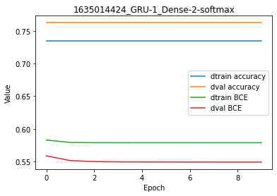
Overall, and using this dummy dataset made of string features, there is no significant metrics/cost difference from the simple Perceptron to recurrent RNN, GRU and LSTM. In this situation, one would favor the simple Perceptron because it computes faster. At least, it is important to note that the best architecture is not the fanciest, but simply the one that suits your needs and resources.
For code, maths and pictures behind the GRU layer, follow this link:
Write, read & Predict
A trained model can be written on disk such as:
[29]:
model.write()

# model.write(path=/your/custom/path)
Make: /media/synthase/beta/EpyNN/epynnlive/dummy_string/models/1635014424_GRU-1_Dense-2-softmax.pickle
A model can be read from disk such as:
[30]:
model = read_model()

# model = read_model(path=/your/custom/path)
We can retrieve new features and predict on them.
[31]:
X_features, _ = prepare_dataset(N_SAMPLES=10)

dset = model.predict(X_features, X_encode=True)
Results can be extracted such as:
[32]:
for n, pred, probs in zip(dset.ids, dset.P, dset.A):
    print(n, pred, probs)
0 1 [0.27207978 0.72792022]
1 1 [0.26511927 0.73488073]
2 1 [0.26579407 0.73420593]
3 1 [0.26865469 0.73134531]
4 1 [0.26554721 0.73445279]
5 1 [0.2699316 0.7300684]
6 1 [0.26448517 0.73551483]
7 1 [0.26460705 0.73539295]
8 1 [0.26701639 0.73298361]
9 1 [0.26556502 0.73443498]