Basics with Perceptron (P)
Find this notebook at
EpyNN/epynnlive/dummy_boolean/train.ipynb.Regular python code at
EpyNN/epynnlive/dummy_boolean/train.py.
Run the notebook online with Google Colab.
Level: Beginner
In this notebook we will review:
Handling Boolean data.
Designing and training a simple perceptron using EpyNN objects.
Basics and general concepts relevant to the context.
This notebook does not enhance, extend or replace EpyNN’s documentation.
Relevant documentation pages for the current notebook:
Import, configure and retrieve data
Follow this link for details about data preparation.
We will import all libraries and configure seeding, behaviors and directory.
Imports
[1]:
# EpyNN/epynnlive/dummy_boolean/train.ipynb
# Install dependencies
!pip3 install --upgrade-strategy only-if-needed epynn

# Standard library imports
import random

# Related third party imports
import numpy as np

# Local application/library specific imports
import epynn.initialize
from epynn.commons.library import (
    configure_directory,
    read_model,
)
from epynn.network.models import EpyNN
from epynn.embedding.models import Embedding
from epynn.dense.models import Dense
from epynnlive.dummy_boolean.prepare_dataset import prepare_dataset
Note that we imported all libraries we will use, at once and on top of the script. Even though we are going through a notebook, we should pay attention to follow good practices for imports as stated in PEP 8 – Style Guide for Python Code.
You may have also noted that # Related third party imports are limited to numpy.
We developed an educational resource for which computations rely on pure Python/NumPy, nothing else.
Configuration
Let’s now proceed with the configuration and preferences for the current script.
[2]:
random.seed(1)

np.set_printoptions(threshold=10)

np.seterr(all='warn')

configure_directory(clear=True)    # This is a dummy example
Remove: /pylibs/EpyNN/epynnlive/dummy_boolean/datasets
Make: /pylibs/EpyNN/epynnlive/dummy_boolean/datasets
Remove: /pylibs/EpyNN/epynnlive/dummy_boolean/models
Make: /pylibs/EpyNN/epynnlive/dummy_boolean/models
Remove: /pylibs/EpyNN/epynnlive/dummy_boolean/plots
Make: /pylibs/EpyNN/epynnlive/dummy_boolean/plots
We already explained the reason for seeding.
The call to np.set_printoptions() set the printing behavior of NumPy arrays. To not overfill this notebook, we instructed that beyond threshold=10 NumPy will trigger summarization rather than full representation.
The call to np.seterr() is very important if you want to be aware of what’s happening in your Network. Follow the numpy.seterr official documentation for details. Herein, we make sure that floating-point errors will always warn on the terminal session and thus we will always be aware of them.
Finally, the call to configure_directory() is purely facultative but creates the default EpyNN subdirectories in the working directory.
Retrieve Boolean features and label
From prepare_dataset we imported the function prepare_dataset().
[3]:
X_features, Y_label = prepare_dataset(N_SAMPLES=50)
Let’s inspect, as always.
[4]:
for sample in list(zip(X_features, Y_label))[:5]:
    features, label = sample
    print(label, (features.count(True) > features.count(False)), features)
1 False [False, True, False, True, True, False, True, False, True, False, False]
0 True [False, True, False, True, True, False, True, False, True, False, True]
0 True [True, True, False, True, False, True, True, False, False, True, False]
1 False [False, False, False, False, False, False, True, True, False, False, True]
1 False [False, False, False, False, False, True, True, False, True, True, True]
We have what we expect. Remember that the conditional expression is the dummy law we used to assign a label to dummy sample Boolean features.
Perceptron - Single layer Neural Network
Herein, we are going to build the most simple Neural Network and train it in the most simple way we can.
The Embedding layer object
In EpyNN, data must be passed as arguments upon call of the Embedding() layer class constructor.
The instantiated object - the embedding or input layer - is always the first layer in Neural Networks made with EpyNN.
[5]:
embedding = Embedding(X_data=X_features,
                      Y_data=Y_label,
                      relative_size=(2, 1, 0)) # Training, validation, testing set
The arguments X_features and Y_label passed in the class constructor have been split with respect to relative_size for training, validation and testing sets.
Let’s take a look at what relative_size means.
[6]:
dataset = list(zip(X_features, Y_label))   # Pair-wise X-Y data

# We print the 10 first only just to not overfill the notebook
for features, label in dataset[:10]:
    print(features, label)
[False, True, False, True, True, False, True, False, True, False, False] 1
[False, True, False, True, True, False, True, False, True, False, True] 0
[True, True, False, True, False, True, True, False, False, True, False] 0
[False, False, False, False, False, False, True, True, False, False, True] 1
[False, False, False, False, False, True, True, False, True, True, True] 1
[False, False, True, True, False, True, True, True, False, True, True] 0
[True, False, False, True, False, False, True, True, False, True, True] 0
[True, True, False, False, True, False, False, True, False, True, True] 0
[True, False, False, False, False, True, True, True, False, True, True] 0
[True, True, False, True, True, True, True, True, False, False, True] 0
Now, we can apply relative_size to split the whole dataset into parts.
[7]:
relative_size=(2, 1, 0)

dtrain_relative, dval_relative, dtest_relative = relative_size

# Compute absolute sizes with respect to full dataset
sum_relative = sum([dtrain_relative, dval_relative, dtest_relative])

dtrain_length = round(dtrain_relative / sum_relative * len(dataset))
dval_length = round(dval_relative / sum_relative * len(dataset))
dtest_length = round(dtest_relative / sum_relative * len(dataset))

# Slice full dataset
dtrain = dataset[:dtrain_length]
dval = dataset[dtrain_length:dtrain_length + dval_length]
dtest = dataset[dtrain_length + dval_length:]
This is the procedure. Let’s see what happened.
[8]:
print(len(dataset))

print(len(dtrain), dtrain_relative)
print(len(dval), dval_relative)
print(len(dtest), dtest_relative)
50
33 2
17 1
0 0
With relative_size=(2, 1, 0) we asked to prepare a training set dtrain two times bigger than the validation set dval.
We have 50 samples.
[9]:
print(50 / 3 * 2)
print(50 / 3 * 1)
33.333333333333336
16.666666666666668
[10]:
print(round(50 / 3 * 2))
print(round(50 / 3 * 1))

print((round(50 / 3 * 2)) == len(dtrain))
print((round(50 / 3 * 1)) == len(dval))
33
17
True
True
Note that since we have set relative_size=(2, 1, 0) the testing set is empty.
Let’s explore some properties and attributes of the instantiated embedding layer object.
[11]:
# Type of object
print(type(embedding))

# Attributes and values of embedding layer
for i, (attr, value) in enumerate(vars(embedding).items()):
    print(i, attr, value)
<class 'epynn.embedding.models.Embedding'>
0 d {}
1 fs {}
2 p {}
3 fc {}
4 bs {}
5 g {}
6 bc {}
7 o {}
8 activation {}
9 se_hPars None
10 se_dataset {'dtrain_relative': 2, 'dval_relative': 1, 'dtest_relative': 0, 'batch_size': None, 'X_scale': False, 'X_encode': False, 'Y_encode': False}
11 dtrain <epynn.commons.models.dataSet object at 0x7f2b28f8d8b0>
12 dval <epynn.commons.models.dataSet object at 0x7f2b28f8dc70>
13 dtest <epynn.commons.models.dataSet object at 0x7f2b28f8d280>
14 dsets [<epynn.commons.models.dataSet object at 0x7f2b28f8d8b0>, <epynn.commons.models.dataSet object at 0x7f2b28f8dc70>]
15 trainable False
Lines 0-9: Inherited from epynn.commons.models.Layer which is the Base Layer. These instance attributes exist for any layers in EpyNN.
Lines 10-15: Instance attributes specific to epynn.embedding.models.Embedding layer.
se_dataset: Contains data-related settings applied upon layer instantiation
(11-13) dtrain, dval, dtest: Training, validation and testing sets in EpyNN
dataSetobject.batch_dtrain: Training mini-batches. Contains the data actually used for training.
dsets: Contains the active datasets that will be evaluated during training. It contains only two
dataSetobjects because dval was set to empty.
The dataSet object
Let’s examine one dataSet object the same way.
[12]:
# Type of object
print(type(embedding.dtrain))

# Attributes and values of embedding layer
for i, (attr, value) in enumerate(vars(embedding.dtrain).items()):
    print(i, attr, value)
<class 'epynn.commons.models.dataSet'>
0 name dtrain
1 active True
2 X [[False  True False ...  True False False]
 [False  True False ...  True False  True]
 [ True  True False ... False  True False]
 ...
 [ True False False ...  True False False]
 [False False False ...  True False  True]
 [False False  True ...  True False  True]]
3 Y [[1]
 [0]
 [0]
 ...
 [1]
 [1]
 [1]]
4 y [1 0 0 ... 1 1 1]
5 b {1: 15, 0: 18}
6 ids [ 0  1  2 ... 30 31 32]
7 A []
8 P []
name: Self-explaining
active: If it contains data
X: Set of sample features
Y: Set of sample label.
y: Set of single-digit sample label.
b: Balance of labels in set.
ids: Sample identifiers.
A: Output of forward propagation
P: Label predictions.
For full documentation of the epynn.commons.models.dataSet object, you can refer to Data - Model.
Note that in the present example we use single-digit labels and therefore the only difference between (3) and (4) is the shape. The reason for this apparent duplicate will appear in a subsequent notebook.
[13]:
print(embedding.dtrain.Y.shape)
print(embedding.dtrain.y.shape)

print(all(embedding.dtrain.Y.flatten() == embedding.dtrain.y))
(33, 1)
(33,)
True
We described how to instantiate the embedding - or input - layer with EpyNN and we browsed the attached attribute-value pairs.
We observed that it contains dataSet objects and we browsed the corresponding attribute-value pairs for the training set.
We introduced all we needed to know.
We are ready.
For more information about these concepts, please follow this link:
The Dense layer object
[14]:
dense = Dense() # Defaults to Dense(nodes=1, activation=sigmoid)
This one was easy. Let’s inspect.
[15]:
# Type of object
print(type(dense))

# Attributes and values of dense layer
for i, (attr, value) in enumerate(vars(dense).items()):
    print(i, attr, value)
<class 'epynn.dense.models.Dense'>
0 d {'u': 1}
1 fs {}
2 p {}
3 fc {}
4 bs {}
5 g {}
6 bc {}
7 o {}
8 activation {'activate': 'sigmoid'}
9 se_hPars None
10 activate <function sigmoid at 0x7f2b28f7baf0>
11 initialization <function xavier at 0x7f2b28f7bca0>
12 trainable True
Note that (1) indicates the number of nodes in the Dense layer, and (8, 11) the activation function for this layer. See Activation - Functions for details.
For code, maths and pictures behind layers in general and the dense layer in particular, follow these links:
The EpyNN Network object
Instantiate your Perceptron
Now that we have an embedding (input) layer and a Dense (output) layer, we can instantiate the EpyNN object which represents the Neural Network.
[16]:
layers = [embedding, dense]
The list layers is the architecture of a Perceptron.
[17]:
model = EpyNN(layers=layers, name='Perceptron_Dense-1-sigmoid')
The object EpyNN is the Perceptron itself.
Let’s prove it.
[18]:
# Type of object
print(type(model))

# Attributes and values of EpyNN model for a Perceptron
for i, (attr, value) in enumerate(vars(model).items()):
    print(i, attr, value)
<class 'epynn.network.models.EpyNN'>
0 layers [<epynn.embedding.models.Embedding object at 0x7f2b28f8d9d0>, <epynn.dense.models.Dense object at 0x7f2b28fb6700>]
1 embedding <epynn.embedding.models.Embedding object at 0x7f2b28f8d9d0>
2 ts 1651394171
3 uname 1651394171_Perceptron_Dense-1-sigmoid
4 initialized False
Does it really contain the layers we instantiated before?
[19]:
print((model.embedding == embedding))
print((model.layers[-1] == dense))
True
True
Perceptron training
It does seem so, yes.
We are going to start the training of this Perceptron with all defaults, the very most simple form.
[20]:
model.train(epochs=100)
--- EpyNN Check ---
Layer: Embedding
compute_shapes: Embedding
initialize_parameters: Embedding
forward: Embedding
shape: (33, 11)
Layer: Dense
compute_shapes: Dense
initialize_parameters: Dense
forward: Dense
shape: (33, 1)
Layer: Dense
backward: Dense
shape: (33, 11)
compute_gradients: Dense
Layer: Embedding
backward: Embedding
shape: (33, 11)
compute_gradients: Embedding
--- EpyNN Check OK! ---
----------------------- 1651394171_Perceptron_Dense-1-sigmoid -------------------------


-------------------------------- Datasets ------------------------------------

+--------+------+-------+-------+
| dtrain | dval | dtest | batch |
|        |      |       | size  |
+--------+------+-------+-------+
| 33     | 17   | None  | None  |
+--------+------+-------+-------+

+----------+--------+------+-------+
| N_LABELS | dtrain | dval | dtest |
|          |        |      |       |
+----------+--------+------+-------+
| 2        | 0: 18  | 0: 9 | None  |
|          | 1: 15  | 1: 8 |       |
+----------+--------+------+-------+

----------------------- Model Architecture -------------------------

+----+-----------+------------+-------------------+-------------+--------------+
| ID | Layer     | Dimensions | Activation        | FW_Shapes   | BW_Shapes    |
+----+-----------+------------+-------------------+-------------+--------------+
| 0  | Embedding | m: 33      |                   | X: (33, 11) | dA: (33, 11) |
|    |           | n: 11      |                   | A: (33, 11) | dX: (33, 11) |
+----+-----------+------------+-------------------+-------------+--------------+
| 1  | Dense     | u: 1       | activate: sigmoid | X: (33, 11) | dA: (33, 1)  |
|    |           | m: 33      |                   | W: (11, 1)  | dZ: (33, 1)  |
|    |           | n: 11      |                   | b: (1, 1)   | dX: (33, 11) |
|    |           |            |                   | Z: (33, 1)  |              |
|    |           |            |                   | A: (33, 1)  |              |
+----+-----------+------------+-------------------+-------------+--------------+

------------------------------------------- Layers ---------------------------------------------

+-------+--------+----------+---------+--------+---------+--------+----------+----------+-----+
| Layer | epochs | schedule | decay_k | cycle  | cycle   | cycle  | learning | learning | end |
|       |        |          |         | epochs | descent | number | rate     | rate     | (%) |
|       |        |          |         |        |         |        | (start)  | (end)    |     |
+-------+--------+----------+---------+--------+---------+--------+----------+----------+-----+
| Dense | 100    | steady   | 0.050   | 0      | 0       | 1      | 0.100    | 0.100    | 100 |
+-------+--------+----------+---------+--------+---------+--------+----------+----------+-----+

+-------+-------+-------+-------------+
| Layer | LRELU | ELU   | softmax     |
|       | alpha | alpha | temperature |
+-------+-------+-------+-------------+
| Dense | 0.300 | 1     | 1           |
+-------+-------+-------+-------------+

----------------------- 1651394171_Perceptron_Dense-1-sigmoid -------------------------


Epoch 99 - Batch 0/0 - Accuracy: 1.0 Cost: 0.05833 - TIME: 5.39s RATE: 1.86e+01e/s TTC: 0s

+-------+----------+----------+-------+--------+-------+---------------------------------------+
| epoch |  lrate   | accuracy |       |  MSE   |       |              Experiment               |
|       |  Dense   |  dtrain  | dval  | dtrain | dval  |                                       |
+-------+----------+----------+-------+--------+-------+---------------------------------------+
|   0   | 1.00e-01 |  0.636   | 0.588 | 0.242  | 0.244 | 1651394171_Perceptron_Dense-1-sigmoid |
|  10   | 1.00e-01 |  0.818   | 0.765 | 0.153  | 0.197 | 1651394171_Perceptron_Dense-1-sigmoid |
|  20   | 1.00e-01 |  0.818   | 0.765 | 0.123  | 0.179 | 1651394171_Perceptron_Dense-1-sigmoid |
|  30   | 1.00e-01 |  0.848   | 0.765 | 0.105  | 0.168 | 1651394171_Perceptron_Dense-1-sigmoid |
|  40   | 1.00e-01 |  0.970   | 0.765 | 0.093  | 0.159 | 1651394171_Perceptron_Dense-1-sigmoid |
|  50   | 1.00e-01 |  1.000   | 0.824 | 0.084  | 0.152 | 1651394171_Perceptron_Dense-1-sigmoid |
|  60   | 1.00e-01 |  1.000   | 0.824 | 0.077  | 0.147 | 1651394171_Perceptron_Dense-1-sigmoid |
|  70   | 1.00e-01 |  1.000   | 0.824 | 0.071  | 0.144 | 1651394171_Perceptron_Dense-1-sigmoid |
|  80   | 1.00e-01 |  1.000   | 0.824 | 0.066  | 0.141 | 1651394171_Perceptron_Dense-1-sigmoid |
|  90   | 1.00e-01 |  1.000   | 0.824 | 0.061  | 0.138 | 1651394171_Perceptron_Dense-1-sigmoid |
|  99   | 1.00e-01 |  1.000   | 0.824 | 0.058  | 0.137 | 1651394171_Perceptron_Dense-1-sigmoid |
+-------+----------+----------+-------+--------+-------+---------------------------------------+
With all defaults, EpyNN returns:
EpyNN Check: Result of a blank epoch to make sure the network is functional. For each layer, output shapes are returned for both the forward and backward propagation.
init_logs: Extended report about datasets, network architecture and shapes.
Evaluation: Real time evaluation of non-empty datasets (may include dtrain, dval, dtest) with default metrics accuracy and default loss function MSE.
See How to use EpyNN - Console for more details.
You may also like to review the Loss - Functions.
For Evaluation and to be straightforward, we want:
Metrics (e.g., accuracy) as high as possible.
Cost (e.g., MSE) as low as possible.
Differences in metrics and cost between training and validation data to be as low as possible, otherwise we talk about overfitting.
Overfitting happens when the model corresponds too closely to a particular set of data.
The terminal report indicates:
Accuracy is 1 or 100% for the training set and 0.824 or 82.4% for the validation set.
MSE is 0.058 and 0.137 for the training and validation set, respectively.
Differences between training and validation data are significant but the model could reproduce the validation data with acceptable accuracy. Still, we are in presence of overfitting.
In the next notebooks, we will see in practice how to reduce overfitting.
Now, we can take the opportunity to define what accuracy means:
[21]:
Y_train = model.embedding.dval.Y  # True labels (i.e. target values)
A_train = model.embedding.dval.A  # Probabilities - Output of model
P_train = model.embedding.dval.P  # Decision from probabilities

for y, a, p in list(zip(Y_train, A_train, P_train))[:10]:
    print(y, a, p)
[0] [0.10853502] [0.]
[0] [0.36626986] [0.]
[1] [0.56927243] [1.]
[1] [0.71776795] [1.]
[1] [0.25847613] [0.]
[0] [0.14270835] [0.]
[1] [0.74599602] [1.]
[0] [0.08445828] [0.]
[1] [0.97949576] [1.]
[1] [0.24478587] [0.]
This print denotes for each row, by column:
The true label or target value: It is
0or1herein.The output probability: The value is within [0, 1]. Therefore, the higher the probability the more confident the model is to predict a label of
1. Conversely, the lower the probability the more confident the model is to predict a label of0.The predicted label or output decision: This is the rounding of the output probability to the nearest integer.
When the number of output nodes is equal to one, rounding of the output probability is as follows:
[22]:
print(all(np.around(A_train) == P_train))
True
Then, the accuracy for each sample is defined as:
[23]:
print((Y_train == P_train))
[[ True]
 [ True]
 [ True]
 ...
 [ True]
 [False]
 [ True]]
Note that the accuracy for each sample is True or False which evaluates to 1 and 0, respectively.
To compute the accuracy with respect to the whole dataset, we need the mean:
[24]:
print((Y_train == P_train).mean())
print(np.around((Y_train == P_train).mean(), 3))
0.8235294117647058
0.824
Note the rounded value is, as expected, identical to the accuracy reported for the last epoch on the validation set.
We can finally plot the results:
[25]:
model.plot(path=False)
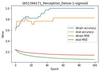
In this plot, dtrain and dval refer to the training and validation set and accuracy/MSE values are identical to those printed on the terminal. This is simply a graphical representation of the tabular log report.
For code, maths and pictures behind the EpyNN model, follow this link:
Write, read & Predict
A trained model can be written on disk such as:
[26]:
model.write()

# model.write(path=/your/custom/path)
Make: /pylibs/EpyNN/epynnlive/dummy_boolean/models/1651394171_Perceptron_Dense-1-sigmoid.pickle
A model can be read from disk such as:
[27]:
model = read_model()

# model = read_model(path=/your/custom/path)
We can retrieve new features and predict on them.
[28]:
X_features, _ = prepare_dataset(N_SAMPLES=10)

dset = model.predict(X_features)
Results can be extracted such as:
[29]:
for n, pred, probs, features in zip(dset.ids, dset.P, dset.A, dset.X):
    print(n, pred, probs, features)
    # pred = output (decision); probs = output (probability)
0 [0.] [0.30108818] [ True False False ...  True  True  True]
1 [0.] [0.14158315] [ True  True  True ...  True False  True]
2 [0.] [0.41840971] [False  True False ...  True  True  True]
3 [0.] [0.08498417] [False  True  True ... False  True  True]
4 [1.] [0.8993867] [ True False  True ...  True False False]
5 [0.] [0.38729994] [False  True False ...  True  True  True]
6 [0.] [0.09610285] [False False  True ... False  True  True]
7 [0.] [0.17566746] [False False  True ... False  True False]
8 [0.] [0.13229161] [ True False  True ...  True  True  True]
9 [0.] [0.15331008] [ True  True  True ...  True  True  True]